
Chapter 4 · 4.4
Conditional formatting: colour cells automatically
With conditional formatting, a cell automatically gets a colour when it meets a condition: a negative amount turns red, an expired date turns orange. In Excel, you find it on the Home tab under Conditional Formatting.
In LibreOffice Calc
- Select the cells.
- Choose Format > Conditional > Condition....
- Choose Cell value, then for example is less than, and enter the value, for example 0.
- Under Apply Style, choose a style, for example Error (red) or Good (green), or create one with New Style....
- Click OK.
The same menu also has Colour Scale..., Data Bar..., Icon Set... and Date.... Use Format > Conditional > Manage... to edit or delete rules.
Colouring a whole row, for example when column D says "paid": select the rows (for example A2:F100), choose Formula is for the condition and type $D2="paid". The dollar sign before the D makes every cell in the row look at column D.
In Euro-Office
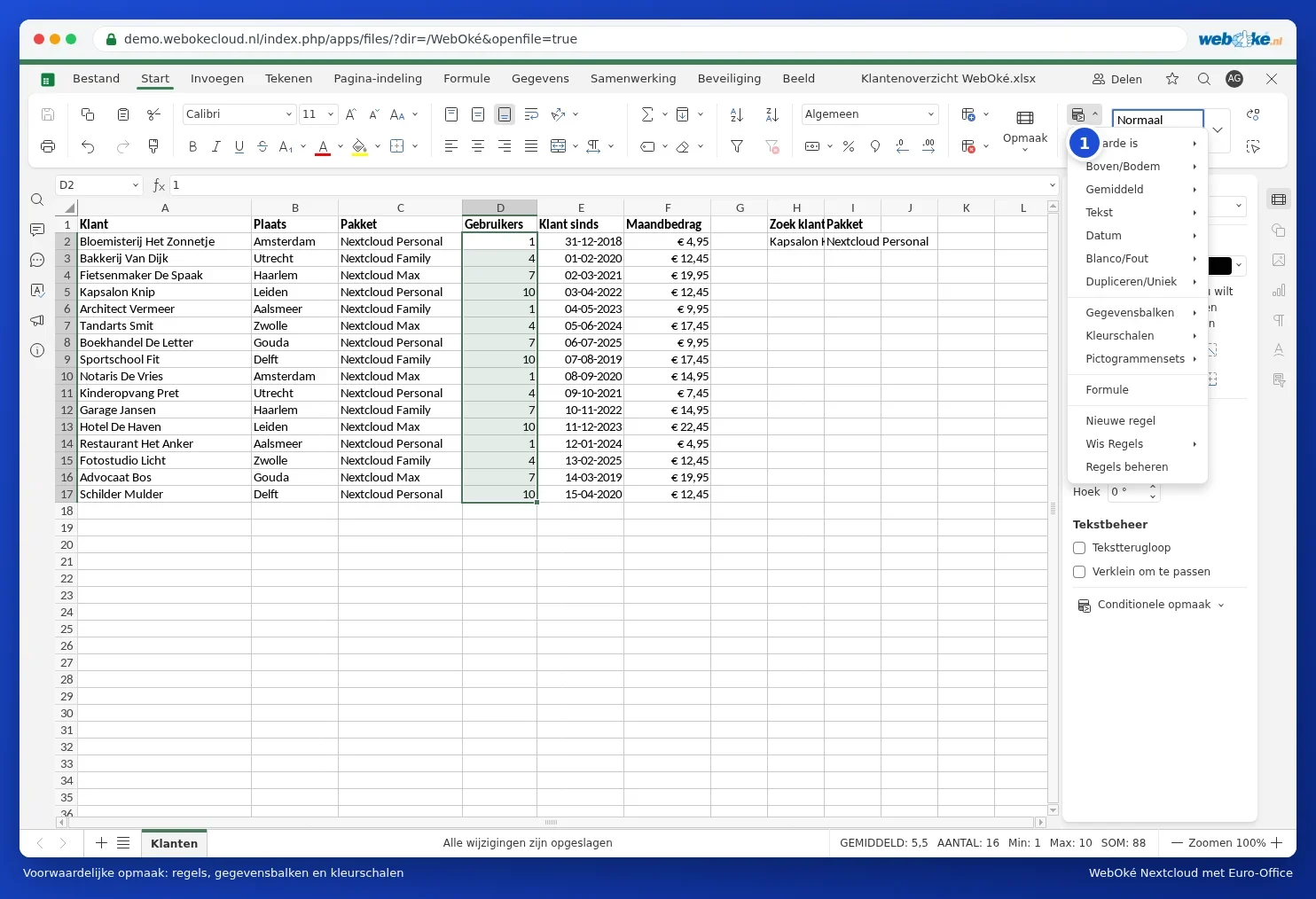
Select the cells and, on the Home tab, click Conditional formatting. Choose a rule and enter the value. Use Manage rules to edit your rules.
Read more in Conditional formatting and see a worked example in Colouring a whole row when the invoice is paid.